hero image

From algorithms to hardware budgets: Estimating and simulating quantum workloads in the Microsoft Quantum Development Kit

Microsoft Quantum Development Kit (QDK) v1.30.0 and QDK for chemistry v2.0.0


by Hariharan Ragunathan, Principal Program Manager and Sasha Schmidt, Principal Program Manager

The answers to two questions determine whether a quantum algorithm is worth pursuing: will it work, and what would it cost to run on real, error-corrected hardware?  Verifying that an algorithm works is often the harder problem, and estimating its cost should be done with as much accuracy as possible. The Microsoft Quantum Development Kit (QDK) answers both questions. The Quantum Resource Estimator (QRE), a layered, composable engine available as a Python module in the QDK, transforms quantum programs to Pareto-optimal hardware estimates across any qubit technology, error-correction scheme, or hardware you want to compare. Alongside it, an enhanced simulation stack featuring Clifford simulation, direct QIR execution, and local neutral-atom simulation for quantum programs—written in a variety of quantum languages such as Q#, Cirq, OpenQASAM and Qiskit—enable developers to validate and debug algorithms before hardware is available. Combined with end-to-end chemistry workflows, the QDK helps you plan, validate, and compare quantum solutions on the path to fault-tolerant quantum computing.


Download Microsoft’s QDK and QDK for chemistry


Why resource estimation matters

Fault-tolerant quantum computing turns collections of noisy physical qubits into reliable, logical qubits through quantum error correction. That reliability isn't free: error-correction codes drive up the number of physical qubits and increase runtimes. So, for anyone designing or evaluating a quantum algorithm, the practical questions are about cost and scale. How many physical qubits will this need? How long will it run? How do those answers change if the hardware or the application algorithm improves, or if I pick a different error-correction code?


The Microsoft Quantum Resource Estimator answers those questions. Rather than waiting for access to fault-tolerant hardware, you can estimate today what an algorithm would require and compare qubit technologies, error-correction schemes, and hardware assumptions side by side to understand which trade-offs move the needle.


A layered architecture

Resource estimator is now available as a ‘qre’ submodule in the ‘qdk’ Python package. Install it alongside the rest of the toolkit - no Azure account required:


pip install --upgrade "qdk[qre]"


(The legacy estimator in the QDK VS Code extension is being deprecated in favor of this module.)


The defining idea behind the new engine is a layered, composable modeling approach. Instead of one monolithic configuration, you build three independent models and combine them:

  • application model - the quantum computation, such as a Q# program;
  • architecture model - the target hardware, such as gate-based superconducting qubits with specific gate times and error rates;
  • error-correction model - the method to turn physical qubits and operations into logical ones, such as QEC codes and magic state factories.


Because the three layers are fully decoupled, you can swap any one of them without rewriting the others. Want to see how the same algorithm fares on neutral-atom versus Majorana hardware? Change one model. Curious how a different error-correction code shifts the qubit/runtime balance? Change one model. That composability is what makes genuine apples-to-apples comparison possible.


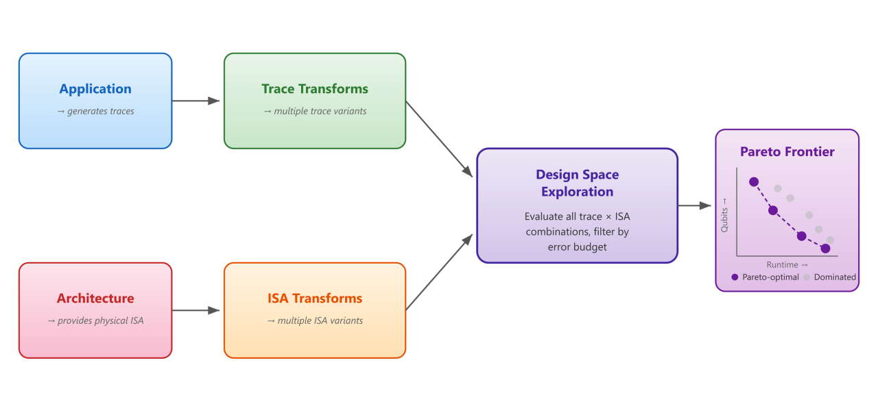
Flowchart showing how application and architecture inputs are processed to explore design options and identify the best tradeoffs.
Start with an application model and an architecture model, derive traces and ISAs, then explore the design space to find the optimal Pareto frontier.


Bring your program in any framework

The estimator is largely framework-agnostic, accepting quantum applications from Q#, Cirq, OpenQASM, QIR, and logical counts. With native QIR support, programs from different quantum ecosystems can flow through the same resource-estimation pipeline.


From built-in models to custom architectures

Resource estimates depend on assumptions about the target hardware and the error-correction code protecting its logical operations. The estimator ships with built-in models for common scenarios and lets you define custom ones to explore hypothetical or emerging architectures. If none of the defaults match what you're studying, you can build custom qubit and error-correction models to evaluate emerging technologies or test how changes in physical parameters ripple through to the resource requirements.


How the engine works under the hood

You interact with the estimator through high-level models, but it's worth understanding what happens beneath them—because the design is what makes the results meaningful.


From the application model, the estimator generates one or more traces: compact representations of the instruction sequences applied to qubits, spanning various implementation choices. From the architecture and error-correction models, it derives a physical instruction set architecture (ISA) specifying operation times, qubit costs, and error rates. Both layers are then turned into configurable transforms—gate decompositions and layout routines on the application side; QEC codes and magic-state factories on the architecture side.


Here's the key: there are many valid choices at each layer—different code distances, factory protocols, and decomposition parameters. For every application trace and architecture ISA combination, the open-source estimator computes physical qubit counts, runtime, and accumulated error. It then selects the Pareto-optimal configurations that deliver the best qubit-runtime tradeoffs while staying within the specified error budget. Learn more on Microsoft Learn: Introduction to the resource estimator Link to Source code & Sample notebooks: github.com/microsoft/qdk , Sample Notebooks  


Exploring hardware trade-offs for quantum chemistry using QRE

Quantum Resource Estimation enables researchers to quickly evaluate hardware requirements of abstract algorithms across different algorithmic primitives and physical systems. QRE is directly integrated with QDK for chemistry, allowing users to go from chemistry problems to quantum algorithms to Pareto-optimal physical resource estimates in a single workflow.


Any circuit generated by the QDK for chemistry library—whether from Trotter evolution, block encoding, or state preparation—can be wrapped as an application model in QRE, making it straightforward for researchers to benchmark an algorithm under different scenarios or conduct parameter sweeps.


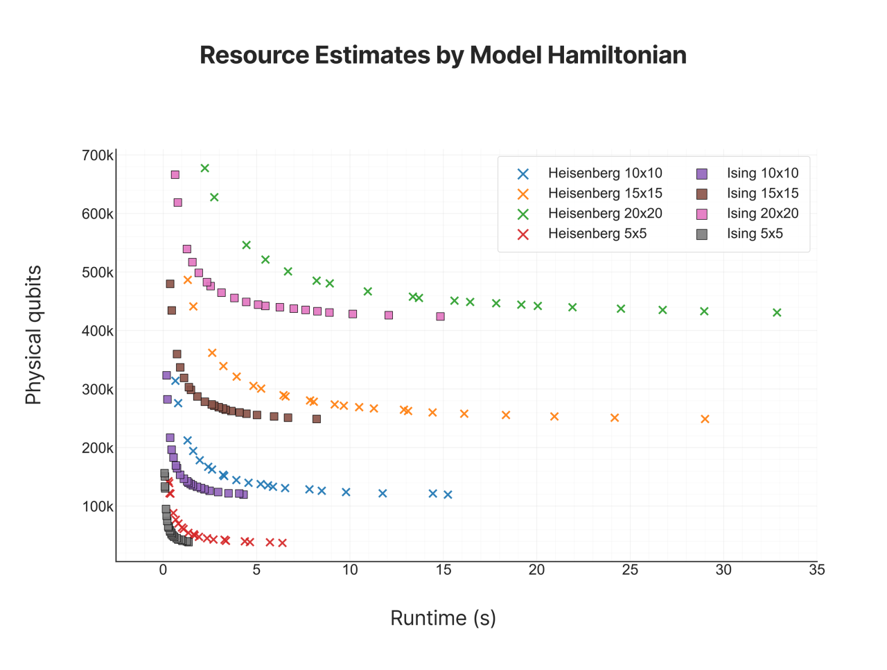
As an example, the QDK estimator can be used to study how physical qubit requirements and runtimes scale with lattice size for different model Hamiltonians.


Chart showing the relationship between runtime and physical qubits for different quantum models.
Pareto-frontier of resources to run a 4th-order Trotter step of 2D Ising model and Heisenberg model across lattice sizes from 5×5 to 20×20 (Majorana-based hardware, with a 1e-5 error rate and ThreeAux error-correction code)


Simulators: Build confidence before running on hardware

Access to real quantum hardware is often limited and costly, so before a single qubit is allocated on a device, you want confidence that your algorithm actually does what you think it does. That's where simulators come in. They let you run, debug, and validate quantum programs entirely in software. While simulation is ultimately limited (classical hardware can only handle a modest number of qubits before the cost grows exponentially) simulators remain an essential tool for validating an algorithm's logic before it ever runs on a real quantum computer.


In the QDK, simulation works alongside the Resource Estimator: the estimator tells you how much quantum hardware an algorithm will eventually need, while simulators confirm the algorithm is correct and behaves as expected long before you commit to hardware. This release makes simulation dramatically more powerful, with three major upgrades.


1. Clifford simulation

When using the Python APIs qdk.qsharp.run or qdk.openqasm.run, you can now pass a type="clifford" argument to run on the Clifford simulator instead of the default sparse simulator. Clifford simulation scales to far higher qubit counts, with the tradeoff that it only supports a restricted set of quantum operations. See the QDK simulators overview for details.


2. Improved simulator capabilities

New Python APIs enable direct execution of QIR on the CPU state vector, Clifford, and GPU state vector simulators, giving developers streamlined access to the underlying simulation engines for testing, debugging, and validation. These simulators now also handle programs generated for the QIR Adaptive Profile, meaning your quantum programs can include mid-circuit measurements, conditional branching, loops, and other adaptive constructs. Check out the QDK Simulators wiki page for the full rundown.


3. Local neutral atom simulation for Cirq and Qiskit

You can now run your Cirq and Qiskit circuits on the local neutral atom simulator. The new NeutralAtomSampler (for Cirq) and NeutralAtomBackend (for Qiskit) let you simulate noisy neutral atom hardware on your own machine, including qubit loss modeling.


For Cirq, the sampler implements cirq.Sampler, so it drops straight into existing Cirq workflows-no rewiring required. Results come back two ways: a standard Cirq-compatible view with loss shots filtered out, and raw data with loss markers for deeper analysis.


For Qiskit, the backend provides a NeutralAtomTarget and automatically transpiles circuits into the native gate set (rz, sx, cz). Walk through it yourself with the neutral atom simulator sample notebook.


Microsoft’s QDK: What's new in QDK v1.30.0

QDK for chemistry: What’s new in QDK for chemistry v2.0.0

Download Microsoft’s QDK and QDK for chemistry